Example 4: Quasi-Monte Carlo

In this example we’ll showcase a useful feature of lintsampler: Quasi-Monte Carlo sampling (QMC).

Quasi-Monte Carlo techniques are a class of sampling algorithms which use low-discrepancy sequences instead of conventional pseudo-random sampling. These sequences are, by construction, more evenly distributed than pseudo-random samples, so that there is less sampling noise for the same number of samples. Some popular examples of such low discrepancy sequences are the Sobol sequence and the Halton sequence.

Python preamble

Imports

import numpy as np
import matplotlib.pyplot as plt
from scipy.stats import multivariate_normal
from lintsampler import LintSampler

Matplotlib style file

plt.style.use('figstyle.mplstyle')

Toy Problem: 2D Gaussian

To demonstrate QMC sampling with lintsampler, we’ll adopt a simple example of a bivariate Gaussian. For the PDF function to feed to LintSampler, we can use the multivariate_normal object from scipy.

mean = np.array([0.5, -1.5])
cov = np.array([[1.5, -0.5],
                [-0.5, 0.5]])
pdf = multivariate_normal(mean, cov).pdf

We’ll also need a coordinate grid to feed to LintSampler:

N_grid = 256
N_s = 2**16
x_edges = np.linspace(-10, 10, N_grid + 1)
y_edges = np.linspace(-10, 10, N_grid + 1)

Basic Usage

To use QMC sampling with lintsampler, simply set the qmc flag to True. To demonstrate this, we’ll take two sets of samples from the PDF, one with QMC and one without.

x0 = LintSampler((x_edges, y_edges), pdf, vectorizedpdf=True).sample(N_s)
x1 = LintSampler((x_edges, y_edges), pdf, vectorizedpdf=True, qmc=True).sample(N_s)

Let’s visualise the two sample sets:

fig = plt.figure(figsize=(10, 4))
ax0 = fig.add_subplot(1, 2, 1)
ax1 = fig.add_subplot(1, 2, 2)
ax0.hist2d(*x0.T, np.linspace(-10, 10, 200));
ax1.hist2d(*x1.T, np.linspace(-10, 10, 200));
ax0.set_title("Default (pseudo-random) sampling")
ax1.set_title("QMC sampling")

for ax in [ax0, ax1]:
    ax.set_xlim(-5, 5)
    ax.set_ylim(-5, 5)

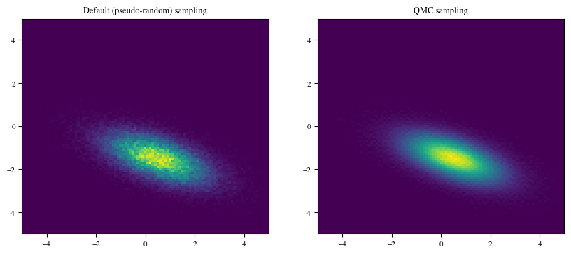
The low-discrepancy set on the right clearly has less sampling noise, as promised.

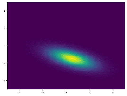
Custom QMC Engines

The default QMC algorithm adopted under the hood here is the scipy implementation of the Sobol sequence: scipy.stats.qmc.Sobol, which is a subclass of the base class scipy.stats.qmc.QMCEngine.

If we instead want to use a different QMC algorithm (or the Sobol sequence with different parameters), we can instance one of the subclasses of QMCEngine and feed that to lintsampler via the qmc_engine parameter.

One thing the user has to be careful of here is in setting the dimensionality of the custom QMCEngine. If sampling from a k-dimensional PDF, the engine should have dimensionality of k+1. This is because, under the hood, the engine draws (N x k+1) uniform samples, uses one column for choosing grid cells and the remainder for lintsampling. In the present problem, we have a bivariate PDF and so need to construct an engine with three dimensions.

Here’s an example using Halton sequencing:

from scipy.stats.qmc import Halton

qmc_engine = Halton(d=3)
x = LintSampler((x_edges, y_edges), pdf, vectorizedpdf=True, qmc=True, qmc_engine=qmc_engine).sample(N_s)

plt.hist2d(*x.T, np.linspace(-10, 10, 200));
plt.xlim(-5, 5)
plt.ylim(-5, 5);

Beware: sample numbers

Another pitfall to be wary of is that the Sobol sequence (the default QMC algorithm in lintsampler) always wants the number of samples to be a power of 2, so a warning is raised if the user requests a number which is not a power of 2. For example:

LintSampler((x_edges, y_edges), pdf, vectorizedpdf=True, qmc=True).sample(10000);

/home/docs/checkouts/readthedocs.org/user_builds/lintsampler/conda/latest/lib/python3.12/site-packages/scipy/stats/_qmc.py:958: UserWarning: The balance properties of Sobol' points require n to be a power of 2.
  sample = self._random(n, workers=workers)

If we wanted to employ QMC sampling but wanted a number of samples which is not a power of 2, we could either:

• Sample more than the desired number then downsample

• Use a different QMC engine (see the example above)