
Error Scaling#
On this page we briefly consider the error scaling of the lintsampling algorithm as applied to Monte Carlo integration.1This page is inspired by a discussion during the JOSS review process (PR #12, in particular this comment by the referee @matt-graham). We’ll use the same toy PDF as in the first example notebook: a 3-component 1D Gaussian mixture. We’ll use lintsampler to get a Monte Carlo estimate of the expectation of the log-pdf,
We can then estimate the ‘error’ as the (absolute) difference between this estimate and a ground truth value.
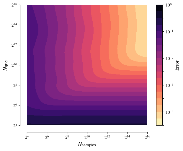
To begin with, we’ll just consider the most ‘vanilla’ usage of lintsampler, i.e. ordinary pseudo-random lintsampling over a single evenly-spaced fixed grid. The plot below shows how the error varies over a two-dimensional space: the number of grid points \(N_\text{grid}\) and the number of samples \(N_\text{samples}\).

The contours here exhibit quite clear L-shapes: holding \(N_\text{samples}\) (\(N_\text{grid}\)) fixed and increasing \(N_\text{grid}\) (\(N_\text{samples}\)), the error decreases rapidly then reaches a plateau at some \(N_\text{grid} < N_\text{samples}\). The key thing to note here is that the error decreases only as \(N_\text{grid}\) and \(N_\text{samples}\) are both increased in tandem.
The following figure repeats this exercise, but now using the quasi-Monte Carlo (QMC) implementation in lintsampler.2This is simply a matter of setting the flag qmc=True in the construction of a LintSampler instance.
Qualitatively, this figure is quite similar to the pseudo-random case above, albeit with two key differences. First, in the QMC case, the error decreases much more quickly as \(N_\text{grid}\) and \(N_\text{samples}\) are increased. Second, the direction of fastest decrease is altered: for a given \(N_\text{grid}\), fewer samples are needed before one reaches the error plateau.
To understand the error scaling in the two cases a little more clearly, we can investigate how the error reduces along the line \(N_\text{grid} = N_\text{samples}\).3We could choose other lines through the \(N_\text{grid}\)-\(N_\text{samples}\) space here, for example the line of steepest descent appears to be approximately \(N_\text{grid} \propto N_\text{samples}^{0.3}\) in the pseudo-random case and \(\propto N_\text{samples}^{0.5}\) in the QMC case. This is shown in the figure below.

As expected, the error decreases more quickly with \(N\) with QMC sampling than without. The slopes is slightly steeper than \(N^{-1}\) in the former case, and approximately \(N^{-0.5}\) in the latter case. These are the expected scalings under the two methods, and we find broadly similar results with different toy problems.