
Worked Example#
This page provides a worked example of drawing a single sample in a situation where we have a (two-dimensional) grid of densities and we would like to draw a sample.1This is not a worked example of using lintsampler (such examples are found in the notebooks elsewhere in the documentation), but a walkthrough of the mathematics covered on the previous page. The first section sets up the simple toy problem with the density grid. The second section shows how to choose a cell within the grid, then the third section shows how to draw a sample within the chosen cell.
Toy Model#
For a toy model, we’ll take a bivariate Gaussian with zero mean and covariance matrix
The contour plot below illustrates this distribution.

Walking outwards from the centre, the four contour lines here are the 1-, 2-, 3-, and 4-\(\sigma\) contours.
Crucially, let’s say we don’t have knowledge of this underlying PDF.2If we did know the underlying PDF, we could (at least in this case) enjoy a much easier life drawing simple Gaussian samples. Instead, we know the densities only at the intersections of the \(16\times 10\) grid shown below.

Along the \(x\) dimension, the 16 cells are not equally sized; the grid has finer \(x\) resolution nearer the origin. Along the \(y\) dimension, the 10 cells are equally sized. This grid geometry was chosen to illustrate an example without a strictly uniform grid. The circles at the grid intersections are coloured by their densities.3The density here is not properly normalised, i.e., the numerical values given (ranging 0 to 16) are merely proportional to the true Gaussian PDF evaluated at the grid intersections.
So, this is our grid of densities, and we want to draw a sample from it.
Cell Choice#
Before drawing a sample, we have to choose a cell from the grid. Having done this, we can then go through the linear interpolant sampling procedure. We went through how to choose a cell in the multiple hyperboxes section of the previous page. To reiterate, we estimate the mass of each cell according to \(V \times \tilde{f}\), where \(V\) is the geometric volume of the cell and \(\tilde{f}\) is the average of the densities at the vertices of the cell.4In this two-dimensional case, for a given rectangular cell \(V\) is simply the area (base times height), and \(\tilde{f}\) is the mean of the four corner densities. We can then get a normalised probability for each cell \(\alpha\) according to
where the sum in the denominator is over all cells in the grid.
The figure below shows all of the cells of the grid, now coloured by their probabilities.
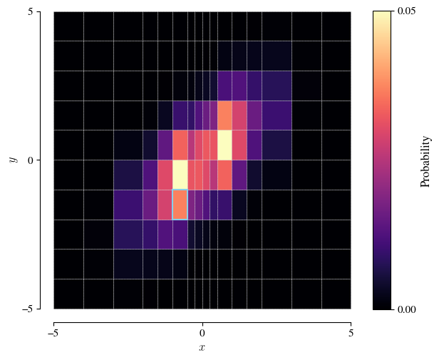
Because of the finer grid resolution close to the origin, the most probable cells are actually two cells centred away from the distribution’s mode.
Given these cell probabilities, we can randomly choose a cell from the probability-weighted list.5For example, in numpy: rng.choice(ncells, p=p), where rng is a numpy random generator, ncells is the (integer) number of cells, and p is the 1D array of cell probabilities (length ncells). In the figure, the cell bordered in blue shows such a choice. We’ll draw a sample within this cell.
Drawing a sample#
Let’s zoom in on the cell we chose above.
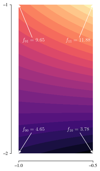
The block fill from the previous figure has been replaced with a colour gradient, showing the bilinear interpolant between the four (labelled) corner densities
Actually, we don’t directly sample from this distribution, but first transform to coordinates \((z_0, z_1)\) so that the cell becomes the unit square. On that domain, the (properly normalised) probability distribution that we’re sampling from is
Now, let’s go through the procedure described on the previous page (summary):
-
6The order in which one cycles through the dimensions does not actually matter; we could start with \(z_1\).
We start with the first dimension (\(z_0\))6The order in which one cycles through the dimensions does not actually matter; we could start with \(z_1\). and calculate the aggregate densities \(g_0\) and \(g_1\). As this is the first dimension, these are simply equal to
\[ g_0 = \tilde{f}_0 = \frac{f_{00} + f_{01}}{2} \approx 7.15 \]\[ g_1 = \tilde{f}_1 = \frac{f_{10} + f_{11}}{2} \approx 7.83 \]Draw a uniform sample \(U_0\). We get a value \(U_0=0.7740\).
Convert \(U_0\) into a sample \(Z_0\) with
\[ Z_0 = \dfrac{-g_0 + \sqrt{g_0^2 + (g_1^2 - g_0^2)U_0}}{g_1 - g_0} \approx 0.78 \]Move on to the second dimension (\(z_1\)) and calculate new aggregate densities \(g_0\) and \(g_1\). This time, these depend on the sample value \(Z_0\) obtained at the first dimension, via
\[ g_0 = f_{00}(1 - Z_0) + f_{10}Z_0 \approx 3.97 \]\[ g_1 = f_{01}(1 - Z_0) + f_{11}Z_0 \approx 11.40 \]Draw a uniform sample \(U_1\). We get a value \(U_1=0.4389\).
Convert \(U_1\) into a sample \(Z_1\) with
\[ Z_1 = \dfrac{-g_0 + \sqrt{g_0^2 + (g_1^2 - g_0^2)U_1}}{g_1 - g_0} \approx 0.56 \]Transform the sample \((Z_0, Z_1)\) from the unit square back to the coordinates of our chosen cell. This is a simple linear (scale and shift) transformation: \(X=-1 + 0.5Z_0\) and \(Y=-2 + Z_1\), giving our final sample \((X, Y)\approx(-0.61, -1.44)\).